
COVID-19 disrupts demand and supply
COVID has impacted economic activity around the world through both demand and supply channels. A combination of higher demand and lower supply of goods has created bottlenecks. These have been discussed at length in the media and by researchers (for example Rees & Rungcharoenkitkul (2021)). The below list outlines some of the factors contributing to this misalignment.
Factors influencing demand and supply throughout COVID-19
Demand
- Substantial fiscal and monetary stimulus supported disposable income and consumption.
- Shift to goods consumption to enable working from home, plus to keep people entertained during lockdowns and away from that on services due to lockdowns. This creates pressure on supply chains as goods involve more component parts.
- Difficulty in securing inventory means firms are buying for precautionary purposes rather than to meet actual demand.
- Demand increases due to peak shopping periods (Black Friday and Christmas) at times when supply was compromised.
Supply
- Firms forecast demand to collapse during the pandemic but instead, it soared. This meant they didn’t produce enough.
- Retailers had moved to running low levels of inventory, which meant that they weren’t able to respond to higher demand.
- Lockdown restrictions reduced production capacity at factories, as well as the availability of port workers and truck drivers.
- Production slowed or ceased due to inability for producers to source inputs.
- Shortage of ships due to lower production prior to COVID.
- Inefficiencies in repositioning empty shipping containers.
- Capital-intensity of manufacturing means it takes longer to expand capacity in response to higher demand.
- Reduction in long-haul passenger flights and thus, on the ability to use freight capacity in the belly of the plane.
- China’s zero COVID strategy has affected production and logistics which is material given its role in global supply chains.
- Border closures affected the availability of skilled labour, which has impacted production.
- Disruptions due to extreme events (for example: weather, fires and power outages at factories, and ships getting stuck in canals).
- Semiconductor supply is restricted, which is delaying manufacturing of other items for which this is an input.
- Russia-Ukraine conflict affecting exports of some items used in auto and semiconductor production.
Source: Various reports from investment banks, Rees & Rungcharoenkitkul (2021)
Indicators of demand and supply
Quantifying demand and supply shocks is difficult. Technical approaches exist but can be quite involved. However, there are other alternatives including news searches, economic data series and simple regression estimates. This section takes a look at some of these to gauge the relative importance of supply and demand factors in driving activity through the COVID shock.
Novel tools have emerged that make it possible to measure economic, market and social developments without relying on traditional data series. One example is Bloomberg News Trends, which allows users to count the number of news articles that mention certain topics. In our case it allows us to capture certain shocks quite nicely (Graph 1).
Graph 1: News-based measures of negative supply (left) and demand (right) shocks for Australia
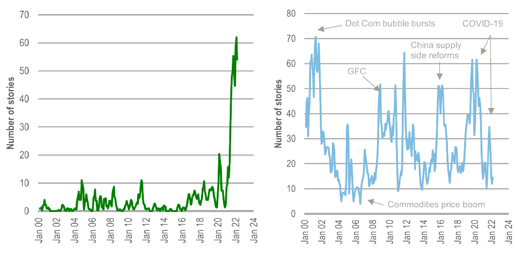
Source: Bloomberg
Note: The left and right charts plot the number of news stories, which mention the topic of ‘supply shortages Australia’ and ‘weak demand Australia’ respectively.
However, these can’t be fully leveraged for our exercise given that it is less obvious what search terms to use for capturing positive supply shocks.1 Given this, I investigated using traditional economic data series to measure demand and supply. Graph 2, which focuses on the manufacturing sector, provides examples of some of the series that have been used as ‘short-hand’ for demand and supply in media and analyst coverage since the onset of the COVID-19 shock.
Graph 2: Economic series, used as ‘short-hand’ measures of demand and supply
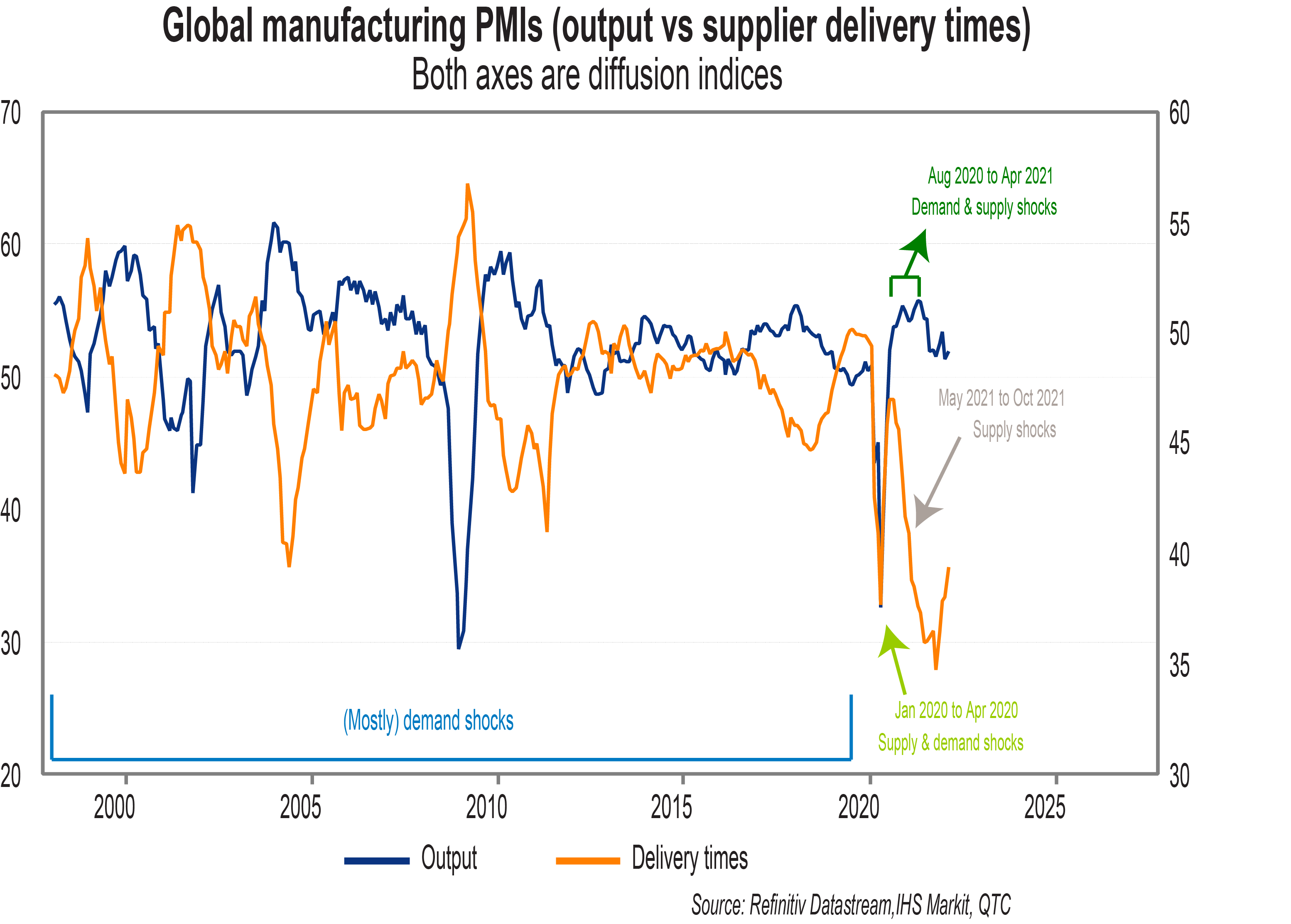
In these sorts of depictions, the output is often cited as a measure of demand and supplier delivery times, a proxy for supply. While this is a neat way to display how the demand and supply have evolved over time, relying on these measures in this way can be problematic as the two series contain both demand and supply elements. For instance, output could fall because of weaker demand or due to a disruption in supply. Similarly, supplier delivery times could increase (the orange line in Graph 1 moves down) due to stronger demand or constrained supply. At any point in time, these ‘short-hand’ measures are influenced by both demand and supply developments.
In the pre-COVID period, the two series typically moved in the opposite direction. For example, higher output (blue line moves up) would coincide with longer delivery times (orange line moves down). This could be interpreted as a demand shock. Since COVID-19, however, the series has moved in ways that suggest a different combination of shocks. At the onset (January to April 2020), shocks to both demand and supply were evident as lockdowns were imposed. As these were unwound (August 2020 to April 2021), demand was quick to rebound but supply less so. This led to the emergence of bottlenecks as capacity constraints were hit. More recently (May to October 2021), supply delivery times have increased as output has faded. This suggests supply shocks have become more prevalent.
Given the influence of both demand and supply on these series, it makes it hard to use the series as tools to describe these concepts. To address this, I estimated proxies for demand and supply using simple regression techniques. This involved firstly identifying indicators of the Australian economy, which could be influenced by both demand and supply. Those selected were the trading conditions, capacity utilisation and purchase costs series from the National Australia Bank (NAB) Business Survey. I then ‘purged’ these series of the influence of demand, by running regressions of these variables on other series, which have a heavy demand component.2
The ‘residuals’ from these regressions represent the portion of the value of these variables, which can’t be explained by these demand-focused indicators. The common trend of these unexplained components was taken as our measure of supply, while the difference between the common trend for all the series being examined and this supply proxy is our measure of demand (Graph 3). This approach is similar in concept to that adopted by New York Fed economists in their Global Supply Chain Pressure Index. The key difference to that analysis is that I focus only on the Australian context and publish estimates for both demand and supply estimates. This is important as it is the interaction between the two that influences economic outcomes.
Graph 3: Demand and supply proxies for Australia
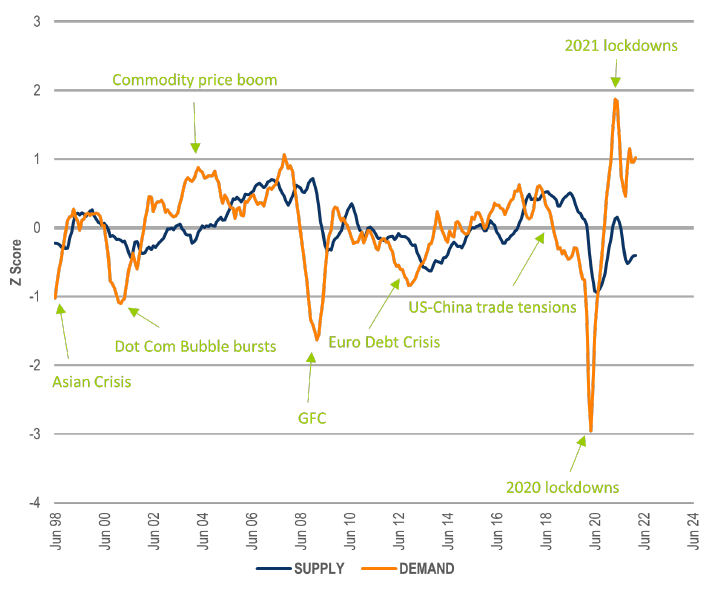
Source: QTC Economic Research, Refinitiv Datastream, Bloomberg, Westpac-ACCI.
These indicators seem to offer a reasonable characterisation of how demand and supply might have evolved over time in Australia. For instance, the movements in demand correspond with key points in the economic cycle over the past two decades. These changes in demand are quicker and more pronounced than for supply. This is what would be expected given inertia in how supply changes.
Just focusing on the changes since the start of COVID-19, the proxy for demand initially fell by more than supply as lockdowns were imposed. As the lockdowns were unwound, demand increased by more than supply. The gap between the two became increasingly pronounced in 2021. This coincided with a spike in media commentary on supply shortages (Graph 1). These of course didn’t occur in isolation, but instead, were heavily influenced by the strong demand. As lockdowns were imposed again later in 2021, demand eased but stayed above supply such that the perceived supply shortages remained. This imbalance has persisted since lockdowns were rolled back in late 2021, as has commentary about supply shortages. As can be observed in this analysis, it is not just the supply side that has driven this phenomenon, but the interaction of strong demand and constrained supply.
So, what impact could these imbalances have on the economic outlook? I take a look at this in the next section with a specific focus on inflation.
How demand and supply imbalances could impact inflation
I examined these demand and supply variables to see how shocks to each impact inflation.3 This could give us a sense of how the shocks being observed at present might impact future inflation outcomes. The results were not conclusive, however.4 As such, it is worth considering what other approaches we could use to get a sense of how the imbalance between demand and supply may impact inflation going forward. I explored two.
Firstly, using the Reserve Bank of Australia (RBA’s) Philip’s Curve inflation model5 my colleague Trent Saunders, QTC Principal Economist, found that the ‘residual’ (that is, the unexplained) component of inflation increased sharply in 2021 with this timing coinciding with when the gap between demand and supply grew as discussed above. Indeed, over 2021 this ‘residual’ has added on average 1.3 percentage points on an annualised basis to trimmed mean inflation (Graph 4). This may capture the demand-supply imbalance to the extent that these pressures can’t be adequately captured by the demand (labour market) and supply (import prices) variables in the model. Equally, it could reflect many other factors including measurement issues and the impact of government support measures. Given the uncertainty around the precise element relating to demand and supply, this should be seen as an upper bound impact.
Graph 4: Drivers of estimated trimmed mean inflation
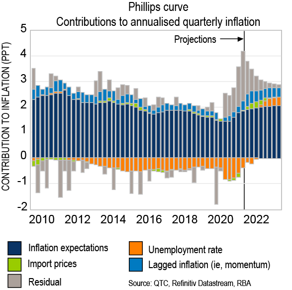
Going forward, and assuming all else is equal, this unexplained component should gradually shrink as the demand‑supply imbalance normalises and the impact of measurement issues and government policy support slowly fade away. One interpretation of the divergence between our inflation forecast and the RBA’s, both constructed using similar models, reflects different judgement as to how quickly this residual normalises. We expect it to be gradual and thus see higher inflation outcomes over the next few years. Our sense is that the RBA expects it to be quicker and thus sees inflation outcomes that are not quite as high.
Secondly, relative to the average levels prior to COVID, businesses have higher inflation expectations over the short‑term (next three months) compared to those of other inflation observers6 (one to two years ahead). One way to reconcile these views is that over the longer-time horizon of the other observers, inflation may moderate from the high levels being expected over the short term by businesses. This could reflect the demand-supply imbalance becoming less pronounced over time. Further, while the current situation is different from others that have been observed previously and alternate outcomes could be realised, it could also be that business’ short-term inflation expectations may not map neatly to what might be observed over longer time horizons. This is consistent with the findings of work that Trent Saunders, QTC Principal Economist, did last year in the article ‘What to expect when you’re expecting inflation.’
Graph 5: Inflation expectations of businesses and other observers
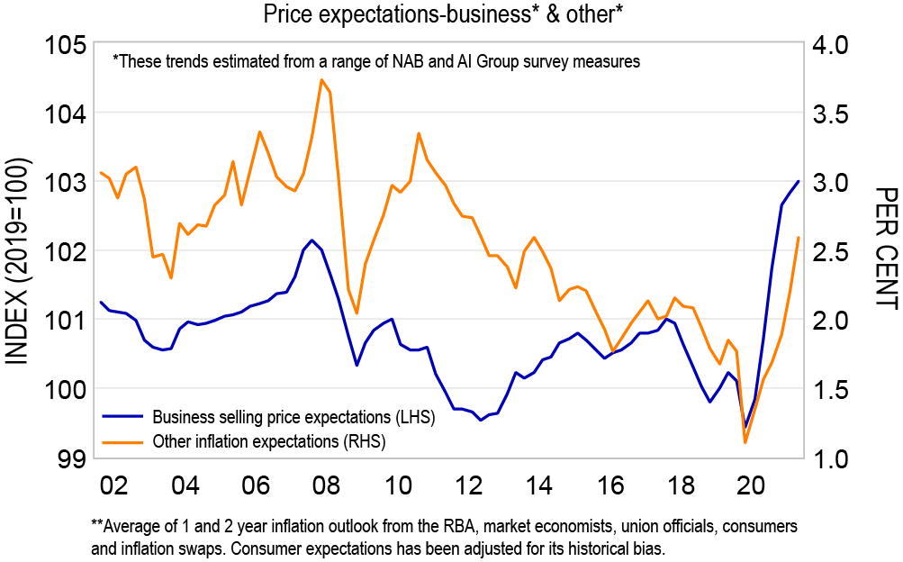
Source: Refinitiv Datastream, ANZ, Bloomberg, RBA, QTC Economic Research
Discussion
An imbalance between demand and supply has emerged as a result of COVID-19. It is challenging to identify how much of this reflects developments on the demand relative to the supply side of the economy. Commonly cited measures are useful for narrative purposes but don’t adequately distinguish between demand and supply influences. I outlined an approach designed to arrive at measures that more cleanly identifies demand and supply. While these measures themselves are not perfect, hopefully they are a useful contribution to better understanding how demand and supply have evolved over time. Going forward, the imbalance is expected to continue to contribute to higher inflation, though it is hard to be precise about the magnitude of this.
Footnotes
(1) For example, there are no news articles over the past couple of decades which mention ‘abundant supply’
(2) These included the series in the Westpac-ACCI Survey which looks at demand being a factor which is limiting production as well as new orders from the NAB Business Survey.
(3) To do so I estimated a vector autoregression with two lags of our supply and demand variables, the cash rate and headline inflation (in that order).
(4) Demand had a positive, significant, and sustained impact on headline inflation. In contrast, supply had a positive, insignificant, and more transitory impact. The insignificance of the supply series could reflect that there have been few substantial swings in supply over the period considered. The results were unsurprisingly less pronounced for trimmed mean inflation given the lower degree of variation in that measure of inflation.
(5) The results are based on the Phillips curve model described by Cassidy et al (2019). The model was estimated using data up to Q4 2019, with the estimated coefficients then being used to calculate the errors from 2020 to 2021. From 2022 onwards, the residual is assumed to decay by around one third each quarter. This results in around 80 per cent of the residual fading away over the four quarters to Q4 2022 and 95 per cent of it fading away by Q4 2023.
(6) These include consumers, unions, the RBA, professional economists, and financial market instruments